Modern Portfolio Theory

We have spent four lessons assembling the pieces:

• diversification;
• correlation;
• position sizing;
• volatility;
• drawdown.

Modern Portfolio Theory walks into the room, looks at all of them, and says:

“Fine. Put everyone in a spreadsheet.”

This is where portfolio construction becomes a formal risk-return problem.

What Is Modern Portfolio Theory?

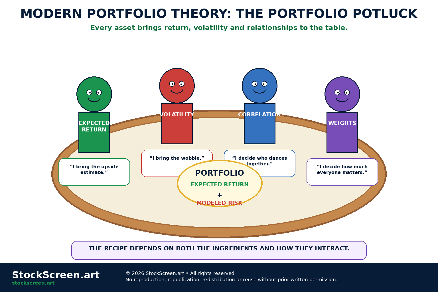
Modern Portfolio Theory (MPT) is a framework for building portfolios by considering expected return, volatility and the way investments move together. Instead of asking whether each asset looks attractive on its own, MPT asks how combinations of assets change the portfolio's overall risk-return profile.

The central insight is that portfolio risk depends not only on the volatility of each holding, but also on correlation and covariance. Assets that do not move perfectly together can sometimes be combined in ways that reduce modeled portfolio volatility without reducing expected return by the same proportion.

A useful beginner framework is: Expected returns → Volatilities → Correlations → Portfolio weights → Feasible set → Efficient frontier → Constraints → Stress test. The model can organize trade-offs, but it cannot guarantee that estimated returns, volatilities or correlations will match the future.

The word together is the important part.

Harry Markowitz's portfolio-selection work changed finance by treating the portfolio itself—not just the individual security—as the object of analysis. His 1952 paper on portfolio selection became foundational to modern financial economics, and he later shared the 1990 Nobel Memorial Prize in Economic Sciences for this work.

1. The pre-Markowitz temptation

Imagine evaluating investments one at a time.

You find Stock A, Stock B and Stock C, each with an attractive expected return.

Obvious conclusion:

“Excellent. Buy all three.”

Missing question:

“How do they behave together?”

2. The portfolio is its own object

A portfolio has properties that cannot be understood by looking at each security separately.

The portfolio has an expected return, volatility, weights, covariance structure and an overall risk-return profile.

It is not merely a folder containing securities.

It is a system.

3. Mean-Variance Analysis in Modern Portfolio Theory

The classic Markowitz framework is often called mean-variance analysis.

• Mean represents expected return.
• Variance or standard deviation represents modeled return dispersion or volatility.

The framework asks how to combine assets to balance those two dimensions.

4. Expected return is not promised return

An expected return is an estimate.

It might come from historical averages, valuation models, economic forecasts, analyst assumptions or capital-market estimates.

None of these creates a contractual promise.

“Expected” is doing a tremendous amount of work in this theory.

5. How Modern Portfolio Theory Calculates Expected Portfolio Return

Expected portfolio return is a weighted average of the expected returns of the assets.

E(Rp) = wA × E(RA) + wB × E(RB)

The weights tell us how much of each asset sits in the portfolio.

6. Simple expected-return example

Fictional assumptions:

• 60% in Asset A with expected return of 8%;
• 40% in Asset B with expected return of 4%.

0.60 × 8% + 0.40 × 4% = 6.4%

The portfolio's expected return is 6.4%.

Again: expected, not scheduled for delivery Tuesday morning.

7. Why portfolio volatility is harder

Expected return is conveniently linear.

Volatility is not.

You cannot generally calculate portfolio volatility by simply taking a weighted average of each asset's volatility, because the assets may not move together.

8. Correlation re-enters the room

From Portfolio Correlation and Overlapping Risk, correlation tells us how return series tend to move together.

Modern Portfolio Theory makes that relationship central. The earlier Portfolio Diversification and Concentration lesson explains the intuition; MPT turns that intuition into a formal portfolio framework.

If two risky assets are not perfectly positively correlated, combining them can reduce portfolio volatility relative to a simple weighted combination of their individual volatilities.

9. Covariance is the portfolio plumbing

Correlation is standardized and easy to read.

Portfolio-variance calculations use covariance.

Cov(A,B) = Correlation(A,B) × σA × σB

Covariance combines the strength of the relationship with each asset's volatility.

10. Two-Asset Portfolio Variance Formula

σp² = wA²σA² + wB²σB² + 2wAwBσAσBρAB

It looks as though the alphabet lost a bar fight.

But conceptually it contains only three ingredients:

1. risk from Asset A;
2. risk from Asset B;
3. how A and B move together.

11. The correlation term is where diversification lives

The final term contains ρAB, the correlation between A and B.

Lower correlation reduces the degree to which the two assets reinforce one another's fluctuations, all else equal.

12. Correlation of +1

If two assets are perfectly positively correlated, they move together in a perfectly linear relationship.

Diversification benefit from combining them is limited.

You have invited two drummers who insist on hitting the same drum at the same time.

13. Correlation below +1

When correlation is less than +1, the assets do not move perfectly together.

This can lower portfolio volatility compared with perfectly correlated assets.

This is the famous diversification effect.

14. Correlation of -1

With perfect negative correlation, it is theoretically possible in a two-asset setup to choose weights that offset variability completely.

Real markets rarely hand out perfect permanent -1 relationships.

Finance is generous with formulas and stingier with ideal conditions.

15. Diversification can improve the risk-return combination

Imagine two assets with similar expected returns but imperfect correlation.

A combination of the two may have similar expected return but lower modeled volatility than either simple intuition might suggest.

The benefit comes from the interaction, not because either asset became safer by itself.

16. Weights create many possible portfolios

With two assets, you can choose many combinations:

• 100% A / 0% B;
• 80% A / 20% B;
• 60% A / 40% B;
• 50% A / 50% B;
• 20% A / 80% B;
• 0% A / 100% B.

Each combination has its own expected return and modeled volatility.

17. Add more assets and the opportunity set expands

With many assets, there can be an enormous number of possible weight combinations.

Plot each possible portfolio using volatility on the horizontal axis and expected return on the vertical axis.

You get a region called the feasible set or opportunity set.

18. The feasible set

The feasible set contains portfolios that can be constructed from the available assets under the rules of the model.

Some portfolios are attractive.

Some are clearly inferior.

Some exist mainly so the optimizer can say:

“Technically, yes. But why?”

19. Dominated portfolios

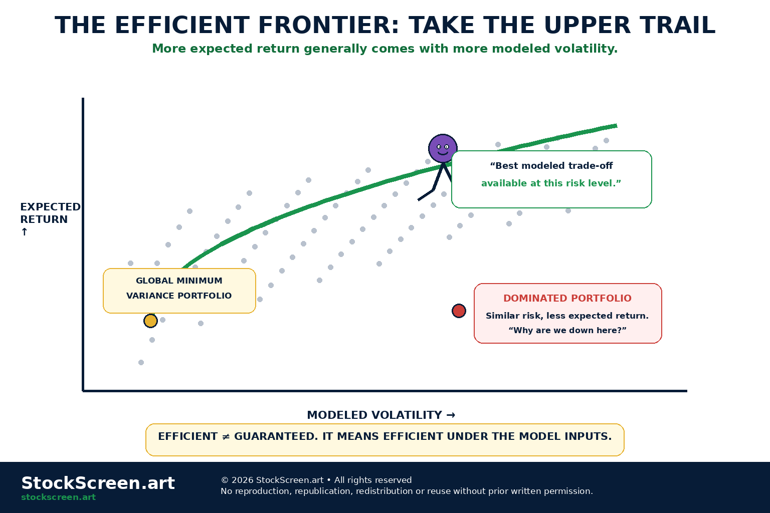
A portfolio is inefficient if another available portfolio offers higher expected return at the same modeled volatility, or lower modeled volatility at the same expected return.

Under those modeled assumptions, the inferior portfolio is dominated.

20. What Is the Efficient Frontier?

The efficient frontier is the upper boundary of the feasible set containing portfolios that provide:

• the highest expected return for a given level of modeled volatility;
• or the lowest modeled volatility for a given expected return.

21. Why the frontier curves

The frontier is not usually a straight line because diversification changes portfolio volatility nonlinearly.

Expected return changes linearly with weights.

Risk depends on weights, volatilities and covariances.

Correlation bends the map.

22. What Is the Global Minimum-Variance Portfolio?

Somewhere on the leftmost edge of the risky-asset opportunity set is the portfolio with the lowest modeled variance.

This is the global minimum-variance portfolio.

It does not necessarily have the lowest expected return.

It has the lowest modeled volatility among the feasible risky portfolios.

23. Below the minimum-variance point

The lower portion of the feasible boundary below the global minimum-variance portfolio is inefficient.

A portfolio on the upper branch offers more expected return for the same modeled risk.

Nobody needs the scenic route to less expected return.

24. “Efficient” does not mean “best for everyone”

Efficient means efficient under the model's risk-return criteria.

Different investors may prefer different points on the frontier because they have different objectives, time horizons, risk tolerances, liquidity needs, tax circumstances and constraints.

25. Investor preference enters after portfolio efficiency

Modern Portfolio Theory separates two questions:

1. Which portfolios are efficient under the assumptions?
2. Which efficient portfolio best fits the investor?

Mathematics can narrow the menu.

It cannot tell every human what to order.

26. Constraints make the model more realistic

Real portfolios often have rules such as:

• no short selling;
• maximum weight per security;
• minimum cash level;
• sector limits;
• tax constraints;
• liquidity requirements;
• minimum or maximum asset-class weights.

These constraints change the feasible set and frontier.

27. An unconstrained optimizer can become weird

Give a mathematical optimizer complete freedom and slightly noisy forecasts, and it may produce huge long positions, huge short positions and tiny weights everywhere else.

The allocation can look like the spreadsheet has personal grievances.

Constraints are often adult supervision.

28. Mean-Variance Optimization: Choosing Portfolio Weights

Mean-variance optimization selects portfolio weights to achieve an objective.

Common objectives include minimizing variance for a target expected return, maximizing expected return for a target variance, or finding the global minimum-variance portfolio.

29. The optimizer does not know the future

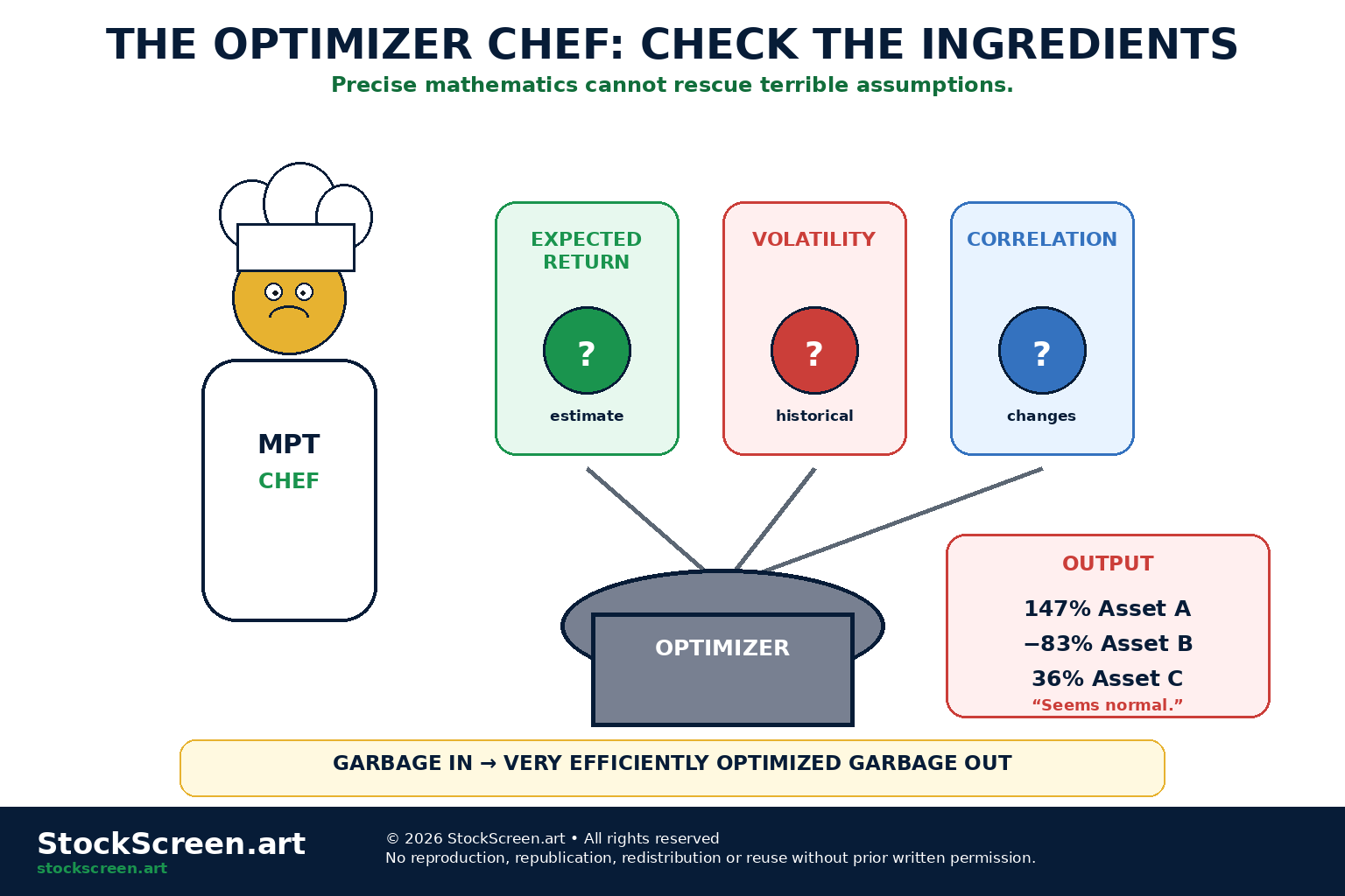
The optimizer knows the inputs you gave it.

Those inputs may include expected returns, volatilities and correlations or covariances.

If those estimates are wrong, the optimizer can be very precisely wrong.

30. Expected returns are especially difficult inputs

Expected returns are notoriously uncertain.

Small changes in expected-return assumptions can sometimes produce large changes in optimized portfolio weights.

This sensitivity is one of the best-known practical problems with mean-variance optimization.

31. Historical averages are noisy

Suppose one asset returned 11% historically and another returned 9%.

That does not prove the first asset's true future expected return is exactly two percentage points higher.

Historical results contain luck, regime effects, valuation changes, one-off events and sampling noise.

32. Volatility estimates are imperfect too

Historical volatility changes over time.

A calm period may underestimate crisis risk.

A crisis-heavy sample may overstate normal conditions.

The model needs a number.

Markets keep changing the answer.

33. Correlation estimates are unstable too

From PR-02, we know correlations can shift across regimes.

A diversification relationship observed in calm markets may weaken during stress.

The covariance matrix is an estimate, not a tablet delivered from the Mountain of Permanent Finance Truths.

34. Garbage in, efficient frontier out

The efficient frontier is mathematically correct for the inputs supplied.

Beautiful optimization charts can be built from bad assumptions.

The curve will still look very professional.

35. Estimation error can produce extreme weights

If the optimizer believes one asset has slightly higher expected return, slightly lower volatility and favourable correlations, it may assign that asset an unexpectedly large weight.

Small input advantages can become large allocation differences.

36. Constraints can reduce estimation sensitivity

Maximum weights, minimum weights and no-short constraints can make optimized portfolios more stable and implementable.

They also mean the result is no longer the unconstrained theoretical optimum.

This is fine.

Real portfolios are allowed to live in the real world.

37. Shrinkage and robust estimation

Professional portfolio construction often uses techniques intended to reduce the effect of noisy estimates.

Examples include shrinking estimates, using factor models, placing limits on weights and testing sensitivity to alternate assumptions.

We do not need the advanced mathematics here.

The lesson is simple:

Do not treat raw estimates as perfect inputs.

38. Equal weighting can be a useful benchmark

An equally weighted portfolio ignores forecasts of expected return.

That sounds unsophisticated.

It also avoids the possibility that tiny forecast differences produce extreme optimization results.

Simple portfolios can be valuable comparison baselines.

39. Minimum variance ignores expected-return estimates

The global minimum-variance portfolio can be constructed using volatility and covariance estimates without requiring explicit expected-return forecasts.

This does not make it perfect.

It simply removes one notoriously noisy input.

40. Risk is not fully captured by variance

Mean-variance analysis treats variance or standard deviation as its main risk measure. The prior Investment Drawdown and Volatility lesson explains why volatility and drawdown are related but not interchangeable risk concepts.

Real investors may also care about drawdown, skewness, tail losses, liquidity, credit risk, permanent impairment and path dependence.

MPT is a powerful framework.

It is not the entire risk-management department.

41. Normal-looking averages can hide ugly tails

Two portfolios can have similar expected return and standard deviation while having very different extreme-loss behavior.

Variance does not tell the whole story about rare events.

42. Nonlinear instruments complicate mean-variance analysis

Options and other nonlinear derivatives can create return distributions that are not well summarized by only mean and variance.

Their risk can change dynamically as market conditions change.

43. Illiquid assets complicate volatility estimates

Assets that trade infrequently can appear artificially smooth because prices are not updated continuously.

Reported volatility may understate economic risk.

A quiet price series is not necessarily a quiet asset.

44. Diversification is not static

Portfolio weights move as prices change.

Volatilities change.

Correlations change.

Expected-return estimates change.

Yesterday's efficient portfolio may not remain efficient under today's assumptions.

45. Rebalancing enters naturally

If a portfolio was built around target weights, market movement will eventually push those weights away from target.

That leads directly to the next lesson: when to restore weights, what rebalancing costs, and how hedging can intentionally reshape exposures.

46. MPT does not say “own everything”

Modern Portfolio Theory does not require owning every possible asset.

It asks how the available assets interact and which combinations are efficient under the assumptions and constraints.

Diversification is purposeful, not a scavenger hunt.

47. MPT does not say “lowest volatility wins”

The global minimum-variance portfolio minimizes modeled volatility.

But investors may reasonably choose more risk in pursuit of higher expected return.

The efficient frontier exists precisely because there is a trade-off.

48. MPT does not say “highest return wins”

Choosing the asset with the highest estimated expected return ignores volatility, correlation, concentration and portfolio interaction.

If expected return were the only input, portfolio theory would be a very short pamphlet.

49. MPT is a language for trade-offs

Its greatest educational value is the discipline of asking:

• What return do I expect?
• What volatility accompanies it?
• How does this asset interact with what I already own?
• Is another portfolio combination more efficient?
• How sensitive is the answer to my assumptions?

50. A Practical Modern Portfolio Theory Workflow

1. Define the investable assets.
2. Estimate expected returns.
3. Estimate volatilities.
4. Estimate correlations or covariances.
5. Define constraints.
6. Generate feasible portfolios.
7. Identify efficient portfolios.
8. Stress-test the assumptions.
9. Compare with simpler benchmarks.
10. Select a portfolio consistent with the investor's actual objectives and risk capacity.

51. Stress-testing the optimizer

Change expected returns slightly.

Change volatility estimates.

Change correlations.

Change the historical sample.

If the portfolio transforms completely after tiny input changes, that instability is important information.

52. Compare the optimized portfolio with simple alternatives

Useful benchmarks can include equal weight, market-cap weight, a simple diversified allocation and the existing portfolio.

Complexity should earn its place.

If a 47-tab workbook produces almost the same answer as “roughly balanced,” the workbook may need a hobby.

53. Seven common MPT mistakes

1. Treating expected returns as facts.
2. Using one historical period and assuming relationships are permanent.
3. Ignoring portfolio constraints.
4. Accepting extreme optimizer weights without investigation.
5. Assuming variance captures every important risk.
6. Confusing an efficient portfolio with a guaranteed profitable portfolio.
7. Adding decimals until uncertainty becomes intimidated.

54. Ten mental models worth keeping

1. Analyze the portfolio, not just the pieces.
2. Expected return is weighted; risk depends on interaction.
3. Correlation is the engine of diversification.
4. The feasible set contains all model-allowed portfolios.
5. The efficient frontier contains the best modeled risk-return combinations.
6. The global minimum-variance portfolio minimizes modeled volatility.
7. Efficient does not mean appropriate for everyone.
8. Optimization is only as good as its inputs.
9. Constraints can make models more realistic and stable.
10. MPT is a framework for disciplined trade-offs, not a future-prediction machine.

Modern Portfolio Theory Questions

What is Modern Portfolio Theory?

Modern Portfolio Theory is a portfolio-construction framework that evaluates expected return, volatility and correlation together. Its core idea is that an investment should be judged partly by how it changes the risk and return of the full portfolio, not only by its standalone characteristics.

What is the efficient frontier?

The efficient frontier is the set of model portfolios that provide the highest expected return for a given level of modeled volatility, or the lowest modeled volatility for a given expected return, under the assumptions and constraints supplied to the model.

What is the global minimum-variance portfolio?

It is the feasible portfolio with the lowest modeled variance or volatility among the available risky-asset combinations. It is not automatically the best portfolio for every investor because investors may choose different levels of risk and expected return.

Why does correlation matter in Modern Portfolio Theory?

Correlation affects how asset returns combine inside the portfolio. When assets are not perfectly positively correlated, their movements can partially offset one another, which can reduce modeled portfolio volatility.

What is the biggest limitation of Modern Portfolio Theory?

MPT depends on estimated expected returns, volatilities and correlations. Those inputs are uncertain and can change through time, so optimized portfolio weights can be unstable or misleading when the assumptions are poor.

Quick knowledge check

Ten questions. The optimizer has been instructed not to assign 147% weight to Question 6.

Where we go next

Modern Portfolio Theory gives us a target portfolio.

Markets immediately begin moving everything away from that target.

Naturally.

So the next lesson is:

FND-PR-06 — Rebalancing and Hedging.

We will look at how portfolio weights drift, when investors may deliberately restore them, and how hedging can reshape risk without pretending the hedge came with a free lunch.

Primary sources & further reading

• NobelPrize.org — Harry M. Markowitz: Facts and Portfolio Selection
• NobelPrize.org — 1990 Prize in Economic Sciences Press Release
• CFA Institute — Portfolio Risk and Return: Part I
• CFA Institute — Portfolio Risk and Return: Part II
• Investor.gov — Beginner's Guide to Asset Allocation, Diversification and Rebalancing