Inside the Training Loop: How an AI Stock-Ranking Model Actually Learns

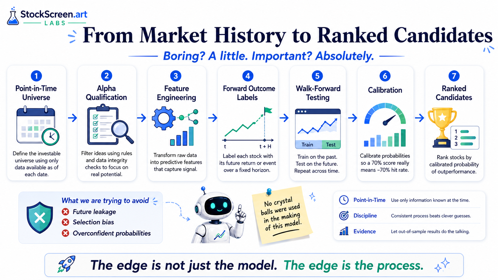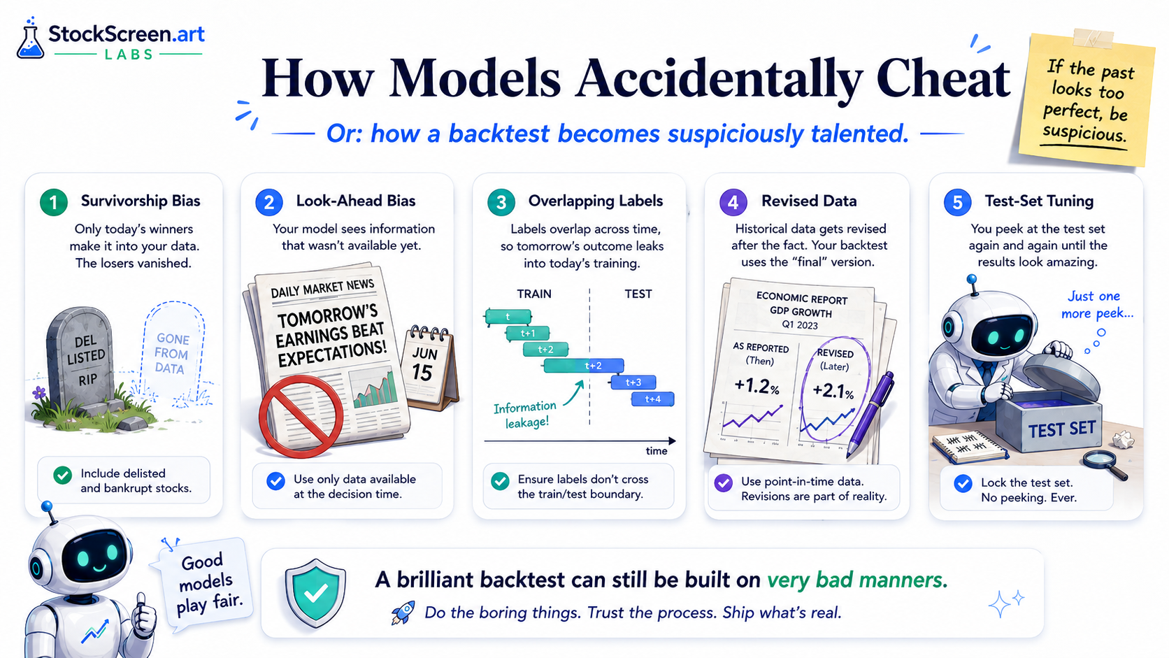
When people hear that an AI model is being trained to identify promising stocks, they often imagine something fairly cinematic.

A wall of market charts. A glowing server. Possibly a robot staring thoughtfully at a candlestick pattern while dramatic music plays in the background.

The real process is less cinematic.

It involves historical tables, date boundaries, feature matrices, validation folds, missing-data checks and an alarming number of files containing words such as final, audit, reconstructed and actually_final.

That may sound less exciting.

It is also where most of the real work happens.

A machine-learning model does not begin by understanding companies, markets or investment risk. It begins with rows and columns.

Each row represents a historical decision that could have been made. Each column contains information that would have been available at that moment. The training process then asks:

When candidates looked like this in the past, what tended to happen next?

The answer is not a prophecy. It is a statistical relationship learned from a carefully constructed historical experiment.

Whether that relationship is useful depends much less on how impressive the algorithm sounds and much more on how the experiment was built.

This article looks inside that process: historical candidate cohorts, feature matrices, outcome labels, purged walk-forward folds, hyperparameter selection, out-of-fold predictions, probability calibration, stability testing, shadow operation and production promotion.

In other words, all the parts that tend to disappear from advertisements containing the phrase “AI-powered stock picks.”

The model does not train on a pile of charts

The model receives a structured training table.

Conceptually, a small portion might look like this:

Cohort date	Ticker	Trend	RSI	Relative strength	ATR %	Alpha score	Forward outcome
2021-03-05	ABC	0.82	56.4	0.17	3.1%	87.2	Success
2021-03-05	XYZ	0.74	63.1	0.09	4.7%	82.6	Failure
2021-03-12	DEF	0.91	51.8	0.24	2.6%	91.4	Success

Each row describes one candidate on one historical selection date.

The same security may appear in several cohorts if it qualified repeatedly. That means these rows are not independent marbles drawn from a bag. They are linked through time, market conditions, company behaviour and sometimes overlapping forward outcomes.

This is one reason ordinary random train/test splitting is inappropriate.

But before reaching the folds, we need to understand where the rows come from.

A cohort is a historical decision room

A cohort is the full set of candidates available to the ranking model on one historical decision date.

Imagine freezing the system on a Friday afternoon in 2022.

The model may know everything legitimately available up to that moment. It may not know what happens the following Monday, which company will surprise the market two weeks later or which stock will become obvious in hindsight.

For that date, the pipeline reconstructs:

1. Which securities existed.
2. Which securities were eligible under the registered universe rules.
3. Which had enough valid historical data.
4. Which passed AlphaEngine qualification.
5. What every permitted feature looked like at that time.
6. What happened during the registered forward outcome period.

That collection becomes one cohort.

The process is repeated across hundreds of dates. In one StockScreen.art reconstruction, the research dataset contained roughly 132,500 Alpha-qualified candidate rows across 640 cohort dates.

A useful mental model is that each cohort represents a separate historical meeting where the system had to choose among the candidates genuinely sitting in the room.

The winners are not allowed to arrive afterward and claim they had been invited all along.

Why the training population must resemble production

MLAlpha is not intended to rank every listed security. AlphaEngine first removes candidates that fail the system’s eligibility, liquidity, trend, volatility and trade-quality standards.

The model therefore trains on the population it will actually see: already-qualified candidates.

Training on the entire market could make the model very good at separating obviously weak securities from obviously stronger ones. That is not the production assignment. AlphaEngine already handles the easy exclusions.

MLAlpha receives the harder population—the stocks that already look reasonably credible—and must learn the differences within that group.

It is the difference between asking which restaurant in the city is good and asking which of twelve well-reviewed restaurants is the best choice tonight.

The second question is narrower. It is also much harder.

Features are snapshots, not biographies

Once a candidate enters a cohort, the pipeline calculates its features.

A feature is a numerical description of what the candidate looked like at that moment. Examples include:

• distance from the 20-, 50- and 200-day moving averages;
• moving-average ordering and trend structure;
• RSI;
• MACD and signal-line relationships;
• average true range as a percentage of price;
• recent realized volatility;
• one-, three- and six-month returns;
• relative strength against an appropriate benchmark;
• liquidity measures;
• expected upside and risk/reward;
• AlphaEngine component scores.

The candidate can be represented as a feature vector:

x_i = [
    RSI,
    MACD,
    ATR percentage,
    one-month return,
    three-month return,
    six-month return,
    relative strength,
    liquidity,
    AlphaEngine components,
    ...
]

The model does not see the chart.

It sees that vector.

The chart is for humans, who remain strangely attached to pictures.

Raw market data needs transformation

Raw price is not directly comparable across securities. A $20 stock and a $400 stock are not meaningfully different simply because one number is larger.

Useful transformations can include:

• returns rather than raw price changes;
• ATR divided by price;
• moving-average distance expressed as a percentage;
• relative rather than absolute performance;
• logarithmic liquidity measures;
• bounded oscillator values;
• rolling standardization fitted only on historical training data.

Every transformation must respect the cohort date.

A rolling 60-day feature may use the preceding 60 days. It may not use thirty days before the decision and thirty days after it because the line looks smoother.

Smoother is not the same as legal.

Missing data needs an explicit contract

Suppose a company has 150 days of price history while the feature set requires a 200-day moving average.

The pipeline needs a registered response:

• exclude the row;
• mark the feature as missing;
• use a defined fallback;
• route the candidate to a shorter-history model;
• postpone eligibility.

What it should not do is insert a convenient number silently and hope nobody asks.

Models are surprisingly tolerant of questionable data decisions.

Auditors are less so.

The target label tells the model what “good” meant

After the feature snapshot is created, the pipeline examines what happened next.

This creates the target label.

For a binary classification problem:

y_i = 1  if the candidate meets the registered success condition
y_i = 0  otherwise

The difficult part is defining the success condition.

A label might use:

• positive return after 21 trading days;
• benchmark outperformance;
• target reached before stop;
• positive net return after estimated costs;
• maximum drawdown remaining below a threshold;
• a combination of return and risk.

For StockScreen.art research, the outcome contract is aligned with how AlphaEngine candidates are intended to be used: a target, a stop and a maximum holding period rather than an open-ended promise that the stock will eventually do something encouraging.

The order of events matters

Suppose both the target and the stop occur within the forward window.

Which happened first?

Daily closing data may not answer that question. Daily high and low may show that both levels were crossed without revealing the intraday order.

The research contract therefore needs a deterministic rule. Options include:

• apply a conservative stop-first assumption;
• use closing-price outcomes only;
• classify same-day collisions as ambiguous;
• exclude ambiguous rows;
• obtain higher-frequency data.

The important point is not that one rule is universally correct.

It is that the rule is explicit and consistent.

Otherwise, every ambiguous case develops a remarkable habit of resolving in favour of the backtest.

Labels create a hidden time interval

Each row has both a decision time and an outcome end time.

If the horizon is 21 trading days, the row occupies an interval:

[decision date, decision date + 21 trading days]

That interval matters when the data is split into folds. A row dated before the test period may still use future prices that extend into the test period.

This is where purging enters the story.

Purging sounds severe.

In this context, it is simply good manners.

Random cross-validation points in the wrong direction

A standard machine-learning tutorial may randomly split observations into training and test groups.

That can work when observations are independent.

Market data is not independent in that way.

A random split could place 2025 observations in training and 2022 observations in testing. It may also place repeated observations for the same company on both sides of the split or allow overlapping forward labels to cross the boundary.

Chronologically, this is ambitious.

Financial validation should move forward through time.

Train on the past. Test on what came next. No time machine.

What a walk-forward fold looks like

An expanding-window design may look like this:

Fold	Training period	Test period
1	2018–2020	2021
2	2018–2021	2022
3	2018–2022	2023
4	2018–2023	2024

Each fold adds more historical data.

A rolling-window design instead forgets older periods:

Fold	Training period	Test period
1	2018–2020	2021
2	2019–2021	2022
3	2020–2022	2023
4	2021–2023	2024

Rolling windows can adapt more quickly when old relationships become stale. They can also discard rare historical environments that may still matter.

There is no universally correct choice. The design depends on data availability, candidate counts, model complexity, expected market drift and the value of older regimes.

The non-negotiable rule is simpler:

The test period must occur after the training period.

This sounds elementary.

A surprising amount of financial machine learning is built on finding elaborate ways around it.

Each fold is a miniature production simulation

Every outer fold should repeat the full pipeline:

1. Select historical training cohorts.
2. Fit preprocessing using training data only.
3. Apply the registered missing-data rules.
4. Train candidate model configurations.
5. Select hyperparameters using inner chronological validation.
6. Retrain on the complete outer training window.
7. Generate predictions for the untouched outer test period.
8. Apply probability calibration without using test outcomes improperly.
9. Rank candidates within each test cohort.
10. Save predictions, diagnostics and versioned artifacts.

The model should not be trained once on the full history and then evaluated on several earlier periods.

That is not walk-forward validation.

That is showing the student the whole textbook before administering several chapter quizzes.

Purging removes answers that cross the boundary

Suppose a fold trains through December 2021 and tests beginning in January 2022.

A training candidate selected on December 20 may have a 21-day outcome label that depends on January prices.

The row belongs to the training period by decision date, but its label reaches into the test period.

The model has therefore learned from part of the future test window.

Purging removes training rows whose outcome intervals overlap the test boundary.

Remove training row i when:

[label start_i, label end_i]
overlaps
[test start, test end]

In plain English:

If a training row needed any part of the test period to know its answer, remove it.

This costs observations.

It also prevents the model from receiving a complimentary sample of the exam answers.

Embargo adds breathing room

Even when labels do not directly overlap, observations close to the boundary may share nearly identical market conditions, feature windows, corporate events or repeated candidate appearances.

An embargo creates a buffer around the boundary.

The correct embargo length depends on the label horizon, feature construction and expected dependence between adjacent cohorts.

A 21-day target generally needs more care than a one-day target.

The purpose is not to make the training and test periods complete strangers.

It is to stop them from quietly sharing notes.

Hyperparameter tuning needs a room inside the room

Models such as XGBoost contain hyperparameters:

• tree depth;
• learning rate;
• number of trees;
• row and column subsampling;
• minimum child weight;
• regularization;
• class weighting.

These settings control flexibility.

A deeper model can capture complicated interactions. It can also memorize historical noise with impressive commitment.

Hyperparameters cannot be selected by repeatedly checking the final test fold.

A safer design uses nested validation:

1. Take the outer fold’s training history.
2. Split that history into smaller inner chronological folds.
3. Train candidate configurations on earlier inner periods.
4. Evaluate them on later inner periods.
5. Select the configuration using only inner results.
6. Retrain that configuration on the full outer training window.
7. Evaluate once on the untouched outer test fold.

The inner folds choose the model.

The outer fold estimates whether the chosen process generalizes.

This is computationally expensive.

It also prevents the final test set from becoming a suggestion box.

Early stopping prevents excessive studying

Gradient-boosted models add trees sequentially.

Performance may improve at first and then deteriorate as the model starts fitting noise.

Early stopping monitors an inner validation period and stops training when improvement has not occurred for a registered number of rounds.

It answers a practical question:

When is the model still learning useful structure, and when has it begun memorizing historical trivia?

Without early stopping, the model may continue adding complexity because nobody told it to go home.

Machines have very poor work-life balance.

Accuracy can be correct and completely useless

Suppose only 25% of qualified candidates meet the success condition.

A model that predicts failure for every candidate achieves 75% accuracy.

It also produces no picks.

Possible responses to class imbalance include:

• class-weighted loss;
• balanced training samples;
• focal loss;
• threshold adjustment;
• ranking-oriented objectives;
• precision-focused evaluation.

Oversampling successful cases can help the model learn minority patterns. It can also duplicate rare examples until they receive more attention than their historical frequency deserves.

Undersampling failures can reduce training cost. It may also discard useful information.

Whatever happens inside training, the outer test folds should preserve the real historical class distribution.

Production will not kindly rebalance the market because training was easier that way.

Classification and ranking are related—but not identical

A classifier estimates whether each candidate belongs to a success class.

A ranking system orders candidates relative to one another.

The model may optimize a classification loss such as log loss:

log loss =
-average[
    y * log(p)
    + (1 - y) * log(1 - p)
]

This rewards probability quality across all rows.

The product, however, may care most about the Top 5 candidates in each weekly cohort.

Useful ranking metrics can include:

• precision at 5;
• hit rate at 5 or 10;
• mean forward return of the Top 5;
• benchmark-relative return;
• normalized discounted cumulative gain;
• pairwise ranking accuracy;
• rank correlation with realized outcomes;
• turnover and downside behaviour.

A model can have good overall log loss while failing to separate the highest-ranked candidates.

Another model may be only modestly better across the full table but much better at identifying the small group the product actually publishes.

The evaluation must match the use case.

Cohort-level metrics stop large weeks from taking over

One historical week may contain 300 qualified candidates while another contains 40.

Pooling all rows gives the large cohort much more influence.

Cohort-level evaluation instead:

1. ranks candidates within each date;
2. selects that date’s Top 5;
3. calculates the cohort result;
4. averages across cohort dates.

This gives each historical decision date a voice.

Otherwise, a few unusually large cohorts can dominate the analysis like someone who has badly misunderstood the purpose of a group discussion.

Out-of-fold predictions are the honest historical record

Each outer test fold produces predictions for rows the model did not train on.

These are out-of-fold predictions.

Combining predictions across all folds creates one historical series where every score came from a model that had not seen that row or any later period.

This out-of-fold dataset supports:

• model comparison;
• probability calibration;
• Top-N evaluation;
• threshold analysis;
• sector and regime analysis;
• error analysis;
• stability testing.

Training-set predictions should not be mixed into this analysis.

Models tend to look excellent on rows they have already seen.

People do too.

That is why open-book exams are labelled differently.

A model score is not automatically a probability

A classifier may produce a number between zero and one.

That does not guarantee the number is a reliable probability.

A model may rank candidates correctly while being overconfident. Candidates scored near 0.70 might succeed only 55% of the time.

Calibration learns a mapping:

raw model score  →  calibrated probability

Common approaches include:

Platt scaling

Fits a logistic transformation to the raw scores. It is smooth and often works well when the calibration relationship is approximately sigmoid-shaped.

Isotonic regression

Learns a flexible monotonic mapping. It can capture irregular calibration curves but may overfit when calibration data is limited.

Beta calibration

Uses a flexible parametric transformation designed for probability outputs.

Whatever method is chosen, calibration must avoid fitting on the outer test fold it is supposed to evaluate.

Otherwise, the score becomes accurate partly because it already knows how the period turned out.

That is less calibration and more revision.

Reliability bins need enough observations

Predicted range	Average prediction	Realized success	Observations
0.40–0.50	0.46	0.44	2,100
0.50–0.60	0.55	0.56	1,840
0.60–0.70	0.64	0.61	920
0.70–0.80	0.74	0.69	310

The highest bin contains fewer observations, so its estimate is less stable.

A system should hesitate before displaying 78.4% when only fourteen genuinely comparable historical cases exist.

The decimal places may be confident.

The evidence is not.

The model should know when today looks unfamiliar

Production candidates may eventually differ from the training population.

Examples include:

• much higher volatility;
• unusual interest-rate conditions;
• new sector leadership;
• different liquidity patterns;
• feature values outside historical ranges;
• a market dominated by a small group of companies.

This is distribution shift.

It can be monitored with:

• population stability index;
• Kolmogorov–Smirnov statistics;
• feature mean and variance drift;
• missing-value rates;
• out-of-range frequencies;
• distance-based support measures;
• changes in the prediction distribution.

The software can still produce a score for an unfamiliar candidate.

Software is helpful that way.

The more important question is whether the score should be trusted.

A responsible system should be able to say that the candidate lies outside the region where the model has strong historical support.

That warning is more useful than another decimal place.

Average performance is not enough

Fold-level results reveal whether a model is broadly useful or dependent on one unusually friendly period.

Compare these two patterns:

• strongly negative, slightly positive, strongly positive, flat;
• moderately positive, moderately positive, moderately positive, moderately positive.

The averages may be similar.

The stability is not.

Each fold should be examined for:

• candidate count and class balance;
• Top-5 and Top-10 hit rates;
• benchmark-relative return;
• drawdown and turnover;
• calibration;
• sector concentration;
• prediction distribution;
• feature importance.

Error analysis looks at the mistakes

False positives are highly ranked candidates that fail. False negatives are candidates the model ranked poorly that succeed.

Repeated questions can reveal useful weaknesses:

• Did the model overvalue short-term momentum?
• Did volatility rise unexpectedly?
• Was liquidity weaker than it appeared?
• Did one sector dominate the errors?
• Was the candidate outside the normal training population?
• Did an event overwhelm the technical evidence?

Error analysis should not produce a custom exception for every historical disappointment.

That road eventually leads to 318 special rules and one deeply concerned maintainer.

Ablation testing makes features earn their place

An ablation test removes one feature or feature group and retrains the model.

Examples:

• remove RSI;
• remove relative strength;
• remove volatility features;
• remove liquidity;
• remove short-term momentum;
• use only AlphaEngine native scores.

If removing a feature changes nothing, the feature may be unnecessary.

If performance improves, it may have been adding noise.

If performance collapses, the model may depend heavily on it—and that dependence should be investigated.

The feature may be genuinely valuable.

It may also be acting as a proxy for time, sector or data availability.

Repeated seeds test training stability

Some algorithms contain randomness through row sampling, column sampling or stochastic optimization.

Training the same configuration with different random seeds can produce different rankings.

Researchers can compare:

• mean and variance of performance;
• Top-5 overlap;
• feature-importance stability;
• calibration stability;
• rank correlation across seeds.

The model does not need to produce identical results every time.

It should not behave as though the random seed is the chief investment officer.

Ensembles may reduce variance

An ensemble can combine:

• several XGBoost models with different seeds;
• models trained on different historical windows;
• tree models and logistic regression;
• regime-specific models;
• calibrated probability averages.

This can reduce sensitivity to one model’s peculiarities.

It also adds storage, inference, calibration and monitoring complexity.

Three mediocre models do not automatically become a genius when placed in a group chat.

The final production model is not the evidence

After the research design is frozen and the chosen configuration has been evaluated across every walk-forward fold, a final production candidate can be trained using all approved history up to the cutoff date.

That final model has now seen the complete approved dataset.

Its training performance is therefore not evidence of generalization.

The out-of-fold results remain the evidence.

The production artifact should include:

• model version;
• training-data cutoff;
• feature schema;
• preprocessing parameters;
• calibration artifact;
• hyperparameters;
• code version;
• data snapshot identifier;
• expected input ranges;
• evaluation report;
• rollback version.

This allows the model to be reproduced by someone other than the person who built it.

Especially if that person is on vacation and their laptop is asleep.

Shadow mode tests the live system

A model can perform well historically and still fail operationally.

Shadow mode runs the model on live data without allowing it to alter published selections.

This tests:

• whether features arrive on time;
• whether data types and units match research;
• whether symbols and sectors map correctly;
• whether candidate counts are plausible;
• whether inference is stable;
• whether probabilities remain calibrated;
• whether rankings become excessively concentrated;
• whether the dashboard receives the expected output.

Shadow mode also records what the model would have selected.

Those selections can later be evaluated using the same target, stop and timeout rules used during training.

This is not another reconstructed backtest.

The system is living through the data as it arrives.

No revisions. No repaired classifications. No convenient knowledge of what happens next.

The model is finally taking the exam under normal supervision.

Promotion requires several kinds of evidence

A challenger should pass explicit gates:

• complete fold coverage;
• no unresolved leakage;
• acceptable calibration;
• stable Top-N results;
• improvement over useful baselines;
• improvement after estimated costs;
• acceptable sector and portfolio concentration;
• reproducible artifacts;
• successful shadow operation;
• rollback readiness.

A result can be statistically positive without being economically meaningful.

It can be economically interesting without being operationally practical.

It can be practical without being stable enough to trust.

Production requires all of those questions to be addressed.

A model that improves one metric by 0.03 percentage points while doubling operational complexity may not be a breakthrough.

It may be a hobby.

Retraining creates a challenger—not an automatic replacement

Markets change, so a production model may eventually need retraining.

The new version should be treated as a challenger.

The current model remains the champion until the challenger demonstrates:

• better or more stable out-of-sample results;
• acceptable calibration;
• consistent Top-N behaviour;
• no harmful concentration;
• successful operational tests;
• a clear rollback path.

A newer training date does not automatically produce a better model.

It produces a newer model.

Software teams have occasionally learned a similar lesson after clicking “Update all.”

Live monitoring continues after deployment

Production monitoring should track:

• feature drift;
• missing-data rates;
• candidate counts;
• prediction and rank distributions;
• sector concentration;
• calibration decay;
• realized target, stop and timeout outcomes;
• unexpected changes after software releases.

A model can underperform temporarily without being broken.

Markets are noisy.

Five disappointing trades are memorable.

Five hundred may deserve a meeting.

The most technical part is discipline

It is tempting to think the hard part is choosing the algorithm.

Often it is not.

XGBoost can be installed with one command.

The difficult work is ensuring that:

• the historical rows are legitimate;
• the universe exists point in time;
• the features use only available information;
• the labels are deterministic;
• the folds move chronologically;
• the boundaries are purged;
• hyperparameters are tuned inside the training window;
• probabilities are calibrated honestly;
• Top-N metrics match the product;
• artifacts are reproducible;
• the production pipeline behaves like the research pipeline.

The model sits in the middle of that system.

It is important.

It is not the whole system.

A powerful algorithm inside a weak experiment produces a sophisticated mistake.

A modest algorithm inside a disciplined experiment can produce useful evidence.

That is why methodology matters.

The goal is not to train a model that looks brilliant in a backtest.

The goal is to train a model that has earned the right to be slightly helpful in the future.

That standard sounds less dramatic.

It is also much harder to fake.

And unlike a suspiciously perfect backtest, it has a reasonable chance of surviving contact with the market.